
Videos
The article “Time Series Analysis for Construction Productivity Experiments” (T. Abdelhamid and J. Everett. Journal of Construction Engineering and Management. 1999:87–95) presents a study comparing the effectiveness of a video system that allows a crane operator to see the lifting point while operating the crane with the old system in which the operator relies on hand signals from a tagman. Three different lifts, A, B, and C, were studied. Lift A was of little difficulty, lift B was of moderate difficulty, and lift C was of high difficulty. Each lift was performed several times, both with the new video system and with the old tagman system. The time (in seconds) required to perform each lift was recorded. The following tables present the means, standard deviations, and
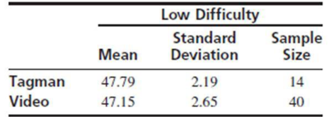
- a. Can you conclude that the mean time to perform a lift of low difficulty is less when using the video system than when using the tagman system? Explain.
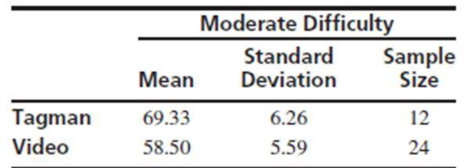
- b. Can you conclude that the mean time to perform a lift of moderate difficulty is less when using the video system than when using the tagman system? Explain.
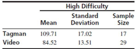
- c. Can you conclude that the mean time to perform a lift of high difficulty is less when using the video system than when using the tagman system? Explain.
a.
Check whether there is evidence to conclude that the mean time to perform a lift of low difficulty is less when using the video system than when using the tagman system.
Answer to Problem 4E
There is no evidence to conclude that the mean time to perform a lift of low difficulty is less when using the video system than when using the tagman system.
Explanation of Solution
Given info:
Three different lifts, A, B, and C, were studied in the given experiment. Lift A was of little difficulty, lift B was of moderate difficulty, and lift C was of high difficulty. The summary statistics for three lifts are given below:
Low difficulty:
Tagman:
Video:
Moderate difficulty:
Tagman:
Video:
High difficulty:
Tagman:
Video:
Calculation:
State the test hypotheses.
Null hypothesis:
Alternative hypothesis:
Tests statistic and P-value:
Software Procedure:
Step-by-step procedure to obtain the test statistic using the MINITAB software:
- Choose Stat > Basic Statistics > 2-Sample t.
- Choose Summarized data.
- In first, enter Sample size as 14, Mean as 47.79, Standard deviation as 2.19.
- In second, enter Sample size as 40, Mean as 47.15, Standard deviation as 2.65.
- Choose Options.
- In Confidence level, enter 95.
- In Alternative, select greater than.
- Click OK in all the dialogue boxes.
Output using the MINITAB software is given below:
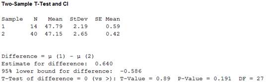
From the MINITAB output, the test statistic is 0.89 and the P-value is 0.191.
Conclusion:
The P-value is 0.191 and the significance level is 0.05.
Here, the P-value is greater than the significance level.
That is,
Therefore, the null hypothesis is not rejected.
Thus, there is no evidence to conclude that the mean time to perform a lift of low difficulty is less when using the video system than when using the tagman system.
b.
Check whether there is evidence to conclude that the mean time to perform a lift of moderate difficulty is less when using the video system than when using the tagman system.
Answer to Problem 4E
There is evidence to conclude that the mean time to perform a lift of moderate difficulty is less when using the video system than when using the tagman system.
Explanation of Solution
Calculation:
State the test hypotheses.
Null hypothesis:
Alternative hypothesis:
Tests statistic and P-value:
Software Procedure:
Step-by-step procedure to obtain the test statistic using the MINITAB software:
- Choose Stat > Basic Statistics > 2-Sample t.
- Choose Summarized data.
- In first, enter Sample size as 12, Mean as 69.33, Standard deviation as 6.26.
- In second, enter Sample size as 24, Mean as 58.50, Standard deviation as 5.59.
- Choose Options.
- In Confidence level, enter 95.
- In Alternative, select greater than.
- Click OK in all the dialogue boxes.
Output using the MINITAB software is given below:
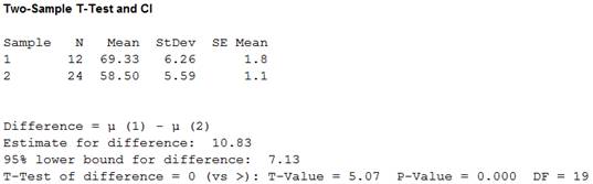
From the MINITAB output, the test statistic is 5.07 and the P-value is 0.000.
Conclusion:
The P-value is 0.000 and the significance level is 0.05.
Here, the P-value is less than the significance level.
That is,
Therefore, the null hypothesis is rejected.
Thus, there is evidence to conclude that the mean time to perform a lift of moderate difficulty is less when using the video system than when using the tagman system.
c.
Check whether there is evidence to conclude that the mean time to perform a lift of high difficulty is less when using the video system than when using the tagman system.
Answer to Problem 4E
There is evidence to conclude that the mean time to perform a lift of high difficulty is less when using the video system than when using the tagman system.
Explanation of Solution
Calculation:
State the test hypotheses.
Null hypothesis:
Alternative hypothesis:
Tests statistic and P-value:
Software Procedure:
Step-by-step procedure to obtain the test statistic using the MINITAB software:
- Choose Stat > Basic Statistics > 2-Sample t.
- Choose Summarized data.
- In first, enter Sample size as 17, Mean as 109.71, Standard deviation as 17.02.
- In second, enter Sample size as 29, Mean as 84.52, Standard deviation as 13.51.
- Choose Options.
- In Confidence level, enter 95.
- In Alternative, select greater than.
- Click OK in all the dialogue boxes.
Output using the MINITAB software is given below:
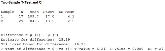
From the MINITAB output, the test statistic is 5.21 and the P-value is 0.000.
Conclusion:
The P-value is 0.000 and the significance level is 0.05.
Here, the P-value is less than the significance level.
That is,
Therefore, the null hypothesis is rejected.
Thus, there is evidence to conclude that the mean time to perform a lift of high difficulty is less when using the video system than when using the tagman system.
Want to see more full solutions like this?
Chapter 6 Solutions
Statistics for Engineers and Scientists
Additional Math Textbook Solutions
Essential Statistics
Business Analytics
Elementary Statistics Using The Ti-83/84 Plus Calculator, Books A La Carte Edition (5th Edition)
Developmental Mathematics (9th Edition)
Essentials of Statistics (6th Edition)
Business Statistics: A First Course (8th Edition)


- Urban Travel Times Population of cities and driving times are related, as shown in the accompanying table, which shows the 1960 population N, in thousands, for several cities, together with the average time T, in minutes, sent by residents driving to work. City Population N Driving time T Los Angeles 6489 16.8 Pittsburgh 1804 12.6 Washington 1808 14.3 Hutchinson 38 6.1 Nashville 347 10.8 Tallahassee 48 7.3 An analysis of these data, along with data from 17 other cities in the United States and Canada, led to a power model of average driving time as a function of population. a Construct a power model of driving time in minutes as a function of population measured in thousands b Is average driving time in Pittsburgh more or less than would be expected from its population? c If you wish to move to a smaller city to reduce your average driving time to work by 25, how much smaller should the city be?arrow_forward4) A study is designed to examine the how the eyes of a model in a magazine advertisement might affect the way a consumer views the product being advertised. Volunteers are assigned one of four ads for a fictional toothpaste, each with a photo of the same model. The only difference is that eyes are digitally made either brown, blue or green OR the model is in the same pose but looking downward so that the eyes are not visible. The variable measured is the viewer's attitude toward the brand. Find the values that go in the boxes for this table. You will enter those values as requested below. ANOVA: Single Factor SUMMARY Groups Blue Brown Green Down ANOVA Source of Variation Between Groups Within Groups Total Q4.1 Box A) Total SS Save Answer Q4.2 Box B) df(num) Save Answer Q4.3 Box C) df(denom) ANOVA: Single Factor SUMMARY Groups Blue Brown Green Down ANOVA Source of Variation Count 67 37 77 41 Between Groups Within Groups SS Total 24.419 613.138 A. Type the value that goes in the box…arrow_forwardQuestion 4 Forys and Dahlquist (2007) investigated the effects of coping style and cognitive strategy on dealing with pain. Participants were first classified as having a monitoring or avoiding coping style. Participants were then randomly assigned to one of two cognitive strategy conditions, distraction or sensation monitoring. Participants were next instructed to use the cognitive strategy while submerging their hand in ice water. The researchers measured pain tolerance as the number of seconds participants were able to keep their hand in the ice water. How would you label the ANOVA used to analyze this data? 4 x 2 within-groups ANOVA O 2x 2 between-groups ANOVA 2 x 2 within-groups ANOVA 4 x 2 between-groups ANOVAarrow_forward
- (2.16) Table 2.12 comes from one of the first studies of the link between lung cancer and smoking, by Richard Doll and A. Bradford Hill. In 20 hospitals in London, UK, patients admitted with lung cancer in the previous year were queried about their smoking behavior. For each patient admitted, researchers studied the smoking behavior of a noncancer control patient at the same hospital of the same sex and within the same 5-year grouping on age. A smoker was defined as a person who had smoked at least one cigarette a day for at least a year. Table 2.12. Data for Problem 2.16 Cases 688 21 709 Lung Cancer Have Smoked Yes No Total Based on data reported in Table IV, R. Doll and A. B. Hill, Br. Med. J., 739-748, September 30, 1950. Controls 650 59 709 a) Identify the response variable and the explanatory variable. b) Identify the type of study this was. c) Can you use these data to compare smokers with nonsmokers in terms of the proportion who suffered lung cancer? Why or why not? d)…arrow_forwardThe article "Combined Analysis of Real-Time Kinematic GPS Equipment and Its Users for Height Determination" (W. Featherstone and M. Stewart, Journal of Surveying Engineering, 2001:31-51) presents a study of the accuracy of global positioning system (GPS) equipment in measuring heights. Three types of equipment were studied, and each was used to make measurements at four different base stations (in the article a fifth station was included, for which the results differed considerably from the other four). There were 60 measurements made with each piece of equipment at each base. The means and standard deviations of the measurement errors (in mm) are presented in the following table for each combination of equipment type and base station. Instrument A Instrument B Instrument C Standard Mean Deviation Mean Deviation Mean Deviation 18 Standard Standard Base 3 15 -24 18 -6 Base 14 26 -13 13 -2 16 Base 26 -22 39 29 Base 34 -17 26 15 18 a Construct an ANOVA table. You may give ranges for the…arrow_forwardWhich model—the one for parliaments or the one for ministries (or cabinets)—presented in the article has the greater explanatory power? How can you tell?arrow_forward
 Calculus For The Life SciencesCalculusISBN:9780321964038Author:GREENWELL, Raymond N., RITCHEY, Nathan P., Lial, Margaret L.Publisher:Pearson Addison Wesley,
 Functions and Change: A Modeling Approach to Coll...AlgebraISBN:9781337111348Author:Bruce Crauder, Benny Evans, Alan NoellPublisher:Cengage Learning
 Linear Algebra: A Modern IntroductionAlgebraISBN:9781285463247Author:David PoolePublisher:Cengage Learning
 Big Ideas Math A Bridge To Success Algebra 1: Stu...AlgebraISBN:9781680331141Author:HOUGHTON MIFFLIN HARCOURTPublisher:Houghton Mifflin Harcourt