
Videos
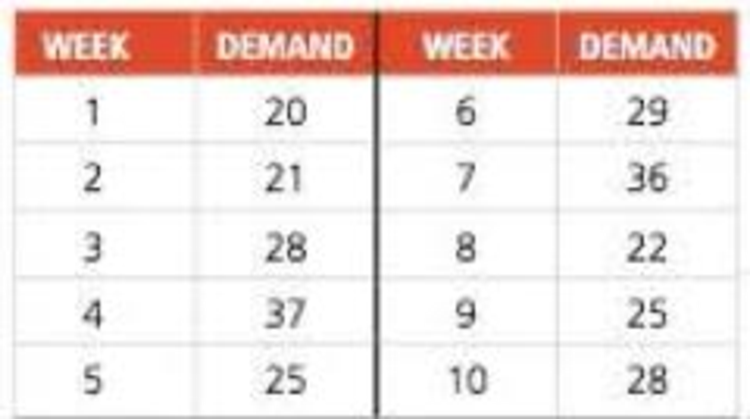
Sales of tablet computers at Ted Glickman’s electronics store in Washington, D.C., over the past 10 weeks are shown in the table below:
a)
b) Compute the MAD.
c) Compute the tracking signal.
a)
To determine: To forecast the demand for 10 weeks using exponential smoothing.
Introduction: A sequence of data points in successive order is known as time series. Time series forecasting is the prediction based on past events, which are at a uniform time interval. Exponential smoothing is one of the time series methods which use a smoothing constant to emphasis past data.
Answer to Problem 59P
Using exponential smoothing, the forecast for week 10 is done.
Explanation of Solution
Given information:
| Week | Demand |
| 1 | 20 |
| 2 | 21 |
| 3 | 28 |
| 4 | 37 |
| 5 | 25 |
| 6 | 29 |
| 7 | 36 |
| 8 | 22 |
| 9 | 25 |
| 10 | 28 |
Formula to calculate the forecasted demand:
Where,
Calculation to forecast demand using exponential smoothing:
| Week | Demand | Ft |
| 1 | 20 | 20 |
| 2 | 21 | 20 |
| 3 | 28 | 20.50 |
| 4 | 37 | 24.25 |
| 5 | 25 | 30.63 |
| 6 | 29 | 27.81 |
| 7 | 36 | 28.41 |
| 8 | 22 | 32.20 |
| 9 | 25 | 27.10 |
| 10 | 28 | 26.05 |
Excel worksheet:
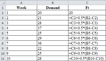
Calculation of the forecast for week 2:
To calculate the forecast for week 2, substitute the value of forecast of week 1, smoothing constant and difference between actual and forecasted demand in the above formula. The result of forecast for week 2 is 20.
Calculation of the forecast for week 3:
To calculate the forecast for week 3, substitute the value of forecast of week 1, smoothing constant and difference between actual and forecasted demand in the above formula. The result of forecast for week 3 is 20.50.
Calculation of the forecast for week 4:
To calculate the forecast for week 4, substitute the value of forecast of week 3, smoothing constant and difference between actual and forecasted demand in the above formula. The result of forecast for week 4 is 24.25.
Calculation of the forecast for week 5:
To calculate the forecast for week 5, substitute the value of forecast of week 4, smoothing constant and difference between actual and forecasted demand in the above formula. The result of forecast for week 5 is 30.63.
Calculation of the forecast for week 6:
To calculate the forecast for week 6, substitute the value of forecast of week 5, smoothing constant and difference between actual and forecasted demand in the above formula. The result of forecast for week 6 is 27.81.
Calculation of the forecast for week 7:
To calculate the forecast for week 7, substitute the value of forecast of week 6, smoothing constant and difference between actual and forecasted demand in the above formula. The result of forecast for week 7 is 28.41.
Calculation of the forecast for week 8:
To calculate the forecast for week 8, substitute the value of forecast of week 7, smoothing constant and difference between actual and forecasted demand in the above formula. The result of forecast for week 8 is 32.20.
Calculation of the forecast for week 9:
To calculate the forecast for week 9, substitute the value of forecast of year 8, smoothing constant and difference between actual and forecasted demand in the above formula. The result of forecast for week 9 is 27.10.
Calculation of the forecast for week 10:
To calculate the forecast for week 10, substitute the value of forecast of year 9, smoothing constant and difference between actual and forecasted demand in the above formula. The result of forecast for week 10 is 26.05.
Thus, using exponential smoothing, the forecast for week 10 is done.
b)
To determine: To compute MAD.
Answer to Problem 59P
MAD is 4.99.
Explanation of Solution
Given information:
| Week | Demand |
| 1 | 20 |
| 2 | 21 |
| 3 | 28 |
| 4 | 37 |
| 5 | 25 |
| 6 | 29 |
| 7 | 36 |
| 8 | 22 |
| 9 | 25 |
| 10 | 28 |
Formula to calculate MAD:
Calculation of MAD:
| Week | Demand | Ft | Absolute error |
| 1 | 20 | 20 | 0 |
| 2 | 21 | 20 | 1 |
| 3 | 28 | 20.50 | 7.50 |
| 4 | 37 | 24.25 | 12.75 |
| 5 | 25 | 30.63 | 5.63 |
| 6 | 29 | 27.81 | 1.19 |
| 7 | 36 | 28.41 | 7.59 |
| 8 | 22 | 32.20 | 10.20 |
| 9 | 25 | 27.10 | 2.10 |
| 10 | 28 | 26.05 | 1.95 |
| Total | 49.91 | ||
| MAD | 4.99 | ||
Table 1
Excel worksheet:
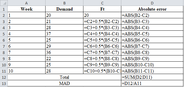
Calculation of the absolute error for week 2:
The absolute error for week 1 is the modulus of the difference between 21 and 20, which corresponds to 1. Therefore, the absolute error for week 2 is 1.
Calculation of the absolute error for week 3:
The absolute error for week 3 is the modulus of the difference between 28 and 20.50, which corresponds to 7.50. Therefore, the absolute error for week 3 is 7.50.
Calculation of the absolute error for week 4:
The absolute error for week 4 is the modulus of the difference between 37 and 24.25, which corresponds to 12.75. Therefore, the absolute error for week 4 is 12.75.
Calculation of the absolute error for week 5:
The absolute error for week 5 is the modulus of the difference between 25 and 30.63, which corresponds to 5.63. Therefore, the absolute error for week 5 is 5.63.
Calculation of the absolute error for week 6:
The absolute error for week 6 is the modulus of the difference between 29 and 27.81, which corresponds to 1.19. Therefore, the absolute error for week 6 is 1.19.
Calculation of the absolute error for week 7:
The absolute error for week 7 is the modulus of the difference between 36 and 28.41, which corresponds to 7.59. Therefore, the absolute error for week 7 is 7.59.
Calculation of the absolute error for week 8:
The absolute error for week 8 is the modulus of the difference between 22 and 32.20, which corresponds to 10.20. Therefore, the absolute error for week 8 is 10.20.
Calculation of the absolute error for week 9:
The absolute error for week 9 is the modulus of the difference between 25 and 27.10, which corresponds to 2.10. Therefore, the absolute error for week 9 is 2.10.
Calculation of the absolute error for week 10:
The absolute error for week 10 is the modulus of the difference between 28 and 26.05, which corresponds to 2.10. Therefore, the absolute error for week 10 is 2.10.
Calculation of the Mean Absolute Deviation:
The substitution of the summation value of absolute error for 10 weeks, divided by the number of weeks, which is 10 yields a MAD of 4.99.
The computed MAD is 4.99.
c)
To determine: To compute the tracking signal.
Answer to Problem 59P
The tracking signal is 2.82.
Explanation of Solution
Given information:
| Week | Demand |
| 1 | 20 |
| 2 | 21 |
| 3 | 28 |
| 4 | 37 |
| 5 | 25 |
| 6 | 29 |
| 7 | 36 |
| 8 | 22 |
| 9 | 25 |
| 10 | 28 |
Formula to calculate tracking signal:
Calculation of tracking signal:
Table 1 shows the calculation of MAD
| Week | Demand | Ft | Absolute error | Error | Cumulative error |
| 1 | 20 | 20 | 0 | 0 | 0 |
| 2 | 21 | 20 | 1 | 1 | 1 |
| 3 | 28 | 20.50 | 7.50 | 7.5 | 8.50 |
| 4 | 37 | 24.25 | 12.75 | 12.75 | 21.25 |
| 5 | 25 | 30.63 | 5.63 | -5.63 | 15.63 |
| 6 | 29 | 27.81 | 1.19 | 1.19 | 16.81 |
| 7 | 36 | 28.41 | 7.59 | 7.59 | 24.41 |
| 8 | 22 | 32.20 | 10.20 | -10.20 | 14.20 |
| 9 | 25 | 27.10 | 2.10 | -2.10 | 12.10 |
| 10 | 28 | 26.05 | 1.95 | 1.95 | 14.05 |
| Total | 49.91 | ||||
| MAD | 4.99 | Tracking signal | 2.82 |
Excel worksheet:
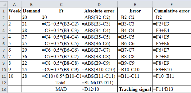
Calculation of tracking signal:
The ratio of cumulative error and MAD is known as the tracking signal. The tracking signal of 2.82 is obtained by dividing 14.05 by 4.99.
Hence, the computed tracking signal is 2.82.
Want to see more full solutions like this?
Chapter 4 Solutions
Principles Of Operations Management


- Under what conditions might a firm use multiple forecasting methods?arrow_forwardThe Baker Company wants to develop a budget to predict how overhead costs vary with activity levels. Management is trying to decide whether direct labor hours (DLH) or units produced is the better measure of activity for the firm. Monthly data for the preceding 24 months appear in the file P13_40.xlsx. Use regression analysis to determine which measure, DLH or Units (or both), should be used for the budget. How would the regression equation be used to obtain the budget for the firms overhead costs?arrow_forwardThe file P13_42.xlsx contains monthly data on consumer revolving credit (in millions of dollars) through credit unions. a. Use these data to forecast consumer revolving credit through credit unions for the next 12 months. Do it in two ways. First, fit an exponential trend to the series. Second, use Holts method with optimized smoothing constants. b. Which of these two methods appears to provide the best forecasts? Answer by comparing their MAPE values.arrow_forward
- The owner of a restaurant in Bloomington, Indiana, has recorded sales data for the past 19 years. He has also recorded data on potentially relevant variables. The data are listed in the file P13_17.xlsx. a. Estimate a simple regression equation involving annual sales (the dependent variable) and the size of the population residing within 10 miles of the restaurant (the explanatory variable). Interpret R-square for this regression. b. Add another explanatory variableannual advertising expendituresto the regression equation in part a. Estimate and interpret this expanded equation. How does the R-square value for this multiple regression equation compare to that of the simple regression equation estimated in part a? Explain any difference between the two R-square values. How can you use the adjusted R-squares for a comparison of the two equations? c. Add one more explanatory variable to the multiple regression equation estimated in part b. In particular, estimate and interpret the coefficients of a multiple regression equation that includes the previous years advertising expenditure. How does the inclusion of this third explanatory variable affect the R-square, compared to the corresponding values for the equation of part b? Explain any changes in this value. What does the adjusted R-square for the new equation tell you?arrow_forwardScenario 4 Sharon Gillespie, a new buyer at Visionex, Inc., was reviewing quotations for a tooling contract submitted by four suppliers. She was evaluating the quotes based on price, target quality levels, and delivery lead time promises. As she was working, her manager, Dave Cox, entered her office. He asked how everything was progressing and if she needed any help. She mentioned she was reviewing quotations from suppliers for a tooling contract. Dave asked who the interested suppliers were and if she had made a decision. Sharon indicated that one supplier, Apex, appeared to fit exactly the requirements Visionex had specified in the proposal. Dave told her to keep up the good work. Later that day Dave again visited Sharons office. He stated that he had done some research on the suppliers and felt that another supplier, Micron, appeared to have the best track record with Visionex. He pointed out that Sharons first choice was a new supplier to Visionex and there was some risk involved with that choice. Dave indicated that it would please him greatly if she selected Micron for the contract. The next day Sharon was having lunch with another buyer, Mark Smith. She mentioned the conversation with Dave and said she honestly felt that Apex was the best choice. When Mark asked Sharon who Dave preferred, she answered, Micron. At that point Mark rolled his eyes and shook his head. Sharon asked what the body language was all about. Mark replied, Look, I know youre new but you should know this. I heard last week that Daves brother-in-law is a new part owner of Micron. I was wondering how soon it would be before he started steering business to that company. He is not the straightest character. Sharon was shocked. After a few moments, she announced that her original choice was still the best selection. At that point Mark reminded Sharon that she was replacing a terminated buyer who did not go along with one of Daves previous preferred suppliers. Ethical decisions that affect a buyers ethical perspective usually involve the organizational environment, cultural environment, personal environment, and industry environment. Analyze this scenario using these four variables.arrow_forwardScenario 4 Sharon Gillespie, a new buyer at Visionex, Inc., was reviewing quotations for a tooling contract submitted by four suppliers. She was evaluating the quotes based on price, target quality levels, and delivery lead time promises. As she was working, her manager, Dave Cox, entered her office. He asked how everything was progressing and if she needed any help. She mentioned she was reviewing quotations from suppliers for a tooling contract. Dave asked who the interested suppliers were and if she had made a decision. Sharon indicated that one supplier, Apex, appeared to fit exactly the requirements Visionex had specified in the proposal. Dave told her to keep up the good work. Later that day Dave again visited Sharons office. He stated that he had done some research on the suppliers and felt that another supplier, Micron, appeared to have the best track record with Visionex. He pointed out that Sharons first choice was a new supplier to Visionex and there was some risk involved with that choice. Dave indicated that it would please him greatly if she selected Micron for the contract. The next day Sharon was having lunch with another buyer, Mark Smith. She mentioned the conversation with Dave and said she honestly felt that Apex was the best choice. When Mark asked Sharon who Dave preferred, she answered, Micron. At that point Mark rolled his eyes and shook his head. Sharon asked what the body language was all about. Mark replied, Look, I know youre new but you should know this. I heard last week that Daves brother-in-law is a new part owner of Micron. I was wondering how soon it would be before he started steering business to that company. He is not the straightest character. Sharon was shocked. After a few moments, she announced that her original choice was still the best selection. At that point Mark reminded Sharon that she was replacing a terminated buyer who did not go along with one of Daves previous preferred suppliers. What should Sharon do in this situation?arrow_forward
- Scenario 4 Sharon Gillespie, a new buyer at Visionex, Inc., was reviewing quotations for a tooling contract submitted by four suppliers. She was evaluating the quotes based on price, target quality levels, and delivery lead time promises. As she was working, her manager, Dave Cox, entered her office. He asked how everything was progressing and if she needed any help. She mentioned she was reviewing quotations from suppliers for a tooling contract. Dave asked who the interested suppliers were and if she had made a decision. Sharon indicated that one supplier, Apex, appeared to fit exactly the requirements Visionex had specified in the proposal. Dave told her to keep up the good work. Later that day Dave again visited Sharons office. He stated that he had done some research on the suppliers and felt that another supplier, Micron, appeared to have the best track record with Visionex. He pointed out that Sharons first choice was a new supplier to Visionex and there was some risk involved with that choice. Dave indicated that it would please him greatly if she selected Micron for the contract. The next day Sharon was having lunch with another buyer, Mark Smith. She mentioned the conversation with Dave and said she honestly felt that Apex was the best choice. When Mark asked Sharon who Dave preferred, she answered, Micron. At that point Mark rolled his eyes and shook his head. Sharon asked what the body language was all about. Mark replied, Look, I know youre new but you should know this. I heard last week that Daves brother-in-law is a new part owner of Micron. I was wondering how soon it would be before he started steering business to that company. He is not the straightest character. Sharon was shocked. After a few moments, she announced that her original choice was still the best selection. At that point Mark reminded Sharon that she was replacing a terminated buyer who did not go along with one of Daves previous preferred suppliers. What does the Institute of Supply Management code of ethics say about financial conflicts of interest?arrow_forwardThe file P13_22.xlsx contains total monthly U.S. retail sales data. While holding out the final six months of observations for validation purposes, use the method of moving averages with a carefully chosen span to forecast U.S. retail sales in the next year. Comment on the performance of your model. What makes this time series more challenging to forecast?arrow_forwardThe manager of a travel agency asked you to come up with a forecasting technique that will best fit to the actual demand for packaged tours. You have observed and recorded the actual demand for the last 10 periods. You also identified two possible techniques for consideration: 2-month moving averages (F1), and exponential smoothing (F2) with a smoothing constant of 0.25. Using Cumulative Forecasting Error (CFE) and Mean Absolute Deviation (MAD) as your performance measures you will determine the technique that will best fit to the actual demand data provided in the following table.STEP 1: Given start forecast values in period 3, compute forecast values from period 4 to 10. You are asked to provide the forecast values for period 6 and 10 for both techniques. 2-Month MA Exponential Period Demand F1 F2 1 115 -- -- 2 176 -- -- 3 97 146 129 4 141 5 98 6 132 7 114 8 129 9 107…arrow_forward
- The number of fishing rods selling each day is given below. Perform analyses of the time series to determine which model should be used for forecasting. 3 day moving average analysis 4 day moving average analysis 3 day weighted moving average analysis with weights W1=0.2, W2=0.3 and W3=0.5 with W1 on the oldest data. Exponential smoothing analysis with A=0.3 Which model provides a better fit of the data? Forecast day 13 sales of fishing rods using the model chosen in part (e) Day Rods Sold 1 60 2 70 3 110 4 80 5 70 6 85 7 115 8 105 9 65 10 75 11 95 12 85 Please read the relevant article, found in the VLE, before answering the question. Discuss the process and findings of the study of the article. Suggest a possible study that could be done at your current or past job that could use a similar methodology and analysis.arrow_forwardSales of Volkswagen's popular Beetle have grown steadily at auto dealerships in Nevada during the past 5 years (see table below). Year Sales 1 450 2 510 3 516 4 563 575 a) Forecasted sales for year 6 using the trend projection (linear regression) method are 613.7 sales (round your response to one decimal place). b) The MAD for a linear regression forecast is sales (round your response to one decimal place).arrow_forwardSales of hair dryers at the NOVO Store in City of San Fernando over the past 4 months have been 100, 110, 120 and 130 units (with 130 being the most recent sales). Develop as moving-average forecast for next month, using these three techniques: a. 3-month moving average b. 4-month moving average. c. Weighted 4-month moving average with the most recent month weighted 4, the preceding month 3, then 2 and the oldest month 1arrow_forward
 Practical Management ScienceOperations ManagementISBN:9781337406659Author:WINSTON, Wayne L.Publisher:Cengage,
 Contemporary MarketingMarketingISBN:9780357033777Author:Louis E. Boone, David L. KurtzPublisher:Cengage Learning
 MarketingMarketingISBN:9780357033791Author:Pride, William MPublisher:South Western Educational Publishing
 Purchasing and Supply Chain ManagementOperations ManagementISBN:9781285869681Author:Robert M. Monczka, Robert B. Handfield, Larry C. Giunipero, James L. PattersonPublisher:Cengage Learning