
Concept explainers
Videos
The article “Photocharge Effects in Dye Sensitized Ag[Br, I] Emulsions at Millisecond
![Chapter 13, Problem 60CR, The article Photocharge Effects in Dye Sensitized Ag[Br, I] Emulsions at Millisecond Range Exposures](https://content.bartleby.com/tbms-images/9781337793612/Chapter-13/images/93612-13-60cr-question-digital_image_001.png)
- a. Construct a
scatterplot of the data. What does it suggest? - b. Assuming that the simple linear regression model is appropriate, obtain the equation of the estimated regression line.
- c. How much of the observed variation in peak photovoltage can be explained by the model relationship?
- d. Predict peak photovoltage when percent absorption is 19.1, and compute the value of the corresponding residual.
- e. The authors claimed that there is a useful linear relationship between the two variables. Do you agree? Carry out a formal test.
- f. Give an estimate of the average change in peak photovoltage associated with a 1 percentage point increase in light absorption. Your estimate should convey information about the precision of estimation.
- g. Give an estimate of mean peak photovoltage when percentage of light absorption is 20, and do so in a way that conveys information about precision.
a.
Construct a scatterplot for the data and explain what it suggests.
Explanation of Solution
Calculation:
The given data are on percentage of light absorption (x) and peak photo voltage (y).
If the scatterplot of the data shows a linear pattern, and the vertical variability of points does not appear to be changing over the range of x values in the sample, then it can be said that the data is consistent with the use of the simple linear regression model.
Software procedure:
Step-by-step procedure to obtain the scatterplot using MINITAB software:
- Choose Graph > Scatter plot.
- Select Simple.
- Click OK.
- Under Y variables, enter the column of y.
- Under X variables, enter the column of x.
- Click OK.
The output using MINITAB software is given below:
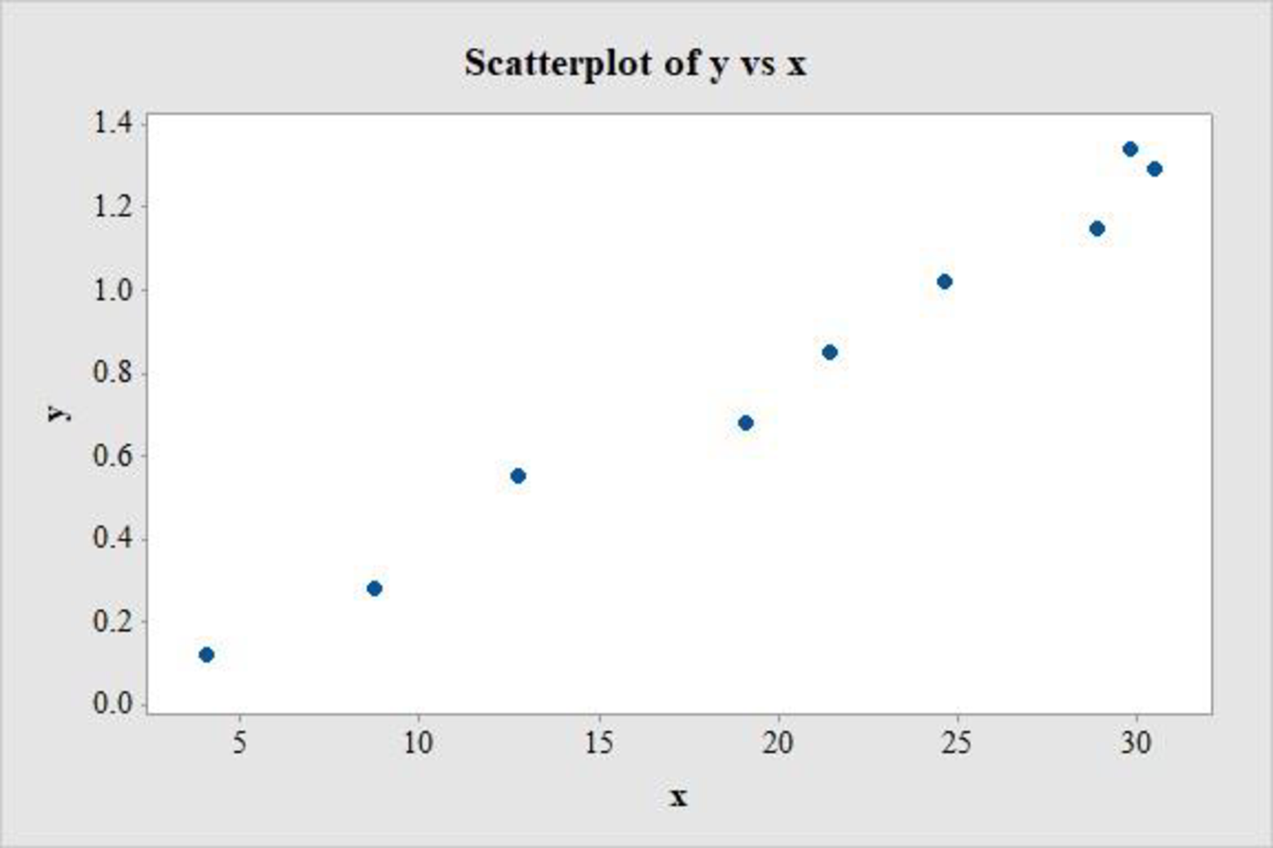
The scatter plot shows no apparent curve and there are no extreme observations. There is no change in the y values as the values of x change and there are no influential points. Therefore, the simple linear regression model seems appropriate for the data set.
b.
Find the equation of the estimated regression line by assuming that the simple linear regression model is appropriate.
Answer to Problem 60CR
The equation of the estimated regression line is,
Explanation of Solution
Calculation:
Regression Analysis:
Software procedure:
Step-by-step procedure to obtain the regression line using MINITAB software:
- Choose Stat > Regression > Regression > Fit Regression Model.
- Under Responses, enter the column of values y.
- Under Continuous predictors, enter the column of values x.
- Click OK.
Output using MINITAB software is given below:
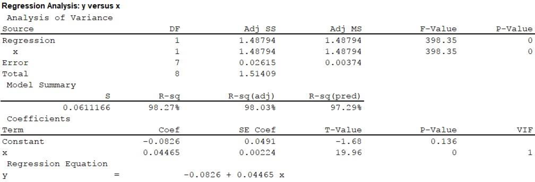
Hence, the equation of the estimated regression line by assuming that the simple linear regression model is appropriate is,
c.
Find how much of the observed variation in peak photo voltage can be explained by the model relationship.
Answer to Problem 60CR
The percentage of observed variation in peak photo voltage that can be explained by the model relationship is 98.3%.
Explanation of Solution
From the Minitab output in Part (b), the value of
This implies that 98.27%, or approximately 98.3% of the observed variation in the dependent variable ‘peak photo voltage’ is being explained by the independent variable ‘percentage of light absorption’ using the simple linear regression model. The change is attributable to the linear relationship between the variables ‘peak photo voltage’ and ‘percentage of light absorption’ and is being explained by the model.
Thus, the percentage of observed variation in peak photo voltage that can be explained by the model relationship is 98.3%.
d.
Predict peak photo voltage when percent absorption is 19.1.
Find the value of the corresponding residual.
Answer to Problem 60CR
The peak voltage when percent absorption is 19.1 is predicted to be 0.770.
The corresponding residual is –0.090.
Explanation of Solution
Calculation:
Predicted value:
The estimated regression equation is,
Hence, the peak voltage when percent absorption is 19.1 is predicted to be 0.770.
Residual:
The formula for residual for response, y and predicted response,
It is given that, when the percentage of light absorption is 19.1, the peak photo voltage is 0.68. Substitute
Hence, the corresponding residual is –0.09.
e.
Explain whether one can agree with the statement that there is a useful linear relationship between the two variables, by carrying out a formal test.
Explanation of Solution
Calculation:
1.
Here,
2.
Null hypothesis:
That is, there is no useful linear relationship between the percentage of light absorption and peak photo voltage.
3.
Alternative hypothesis:
That is, there is a useful linear relationship between the percentage of light absorption and peak photo voltage.
4.
Here, the significance level is assumed to be
5.
Test Statistic:
The formula for test statistic is as follows:
In the formula, b denotes the estimated slope,
6.
Assumption:
The assumption made in Part (b) is that, the simple linear regression model is appropriate.
7.
Calculation:
From the MINITAB output in Part (b), the t-test statistic value for
8.
P-value:
From the MINITAB output in Part (b), the P-value is 0.
9.
Decision rule:
- If P-value is less than or equal to the level of significance, reject the null hypothesis.
- Otherwise, fail to reject the null hypothesis.
10.
Conclusion:
The P-value is 0.
The level of significance is 0.05.
The P-value is less than the level of significance.
That is,
Based on rejection rule, reject the null hypothesis.
Thus, there is convincing evidence of a useful relationship between the percentage of light absorption and peak photo voltage at the 0.05 level of significance.
f.
Obtain an estimate of the average change in peak photo voltage associated with a 1 percentage point increase in light absorption.
Answer to Problem 60CR
The estimate of the average change in peak photo voltage associated with a 1 percentage point increase in light absorption is between 0.039 and 0.050.
Explanation of Solution
Calculation:
From the MINITAB output in Part (b), the value of slope is approximately
Formula for Degrees of freedom:
The formula for degrees of freedom is,
In the formula, n is the total number of observations.
Formula for Confidence interval for
In the formula b denotes the estimated slope and
Degrees of freedom:
The number of data values given are 9, that is
From the Appendix: Table 3 t Critical Values:
- Locate the value 7 in the degrees of freedom (df) column.
- Locate the 0.95 in the row of central area captured.
- The intersecting value that corresponds to the df 7 with confidence level 0.95 is 2.37.
Thus, the critical value for
Confidence interval:
Substitute,
Hence, the 95% confidence interval for estimating the average change in peak photo voltage associated with a 1 percentage point increase in light absorption is
Interpretation:
The 95% confidence interval can be interpreted as: there is 95% confidence that the mean increase in peak photo voltage associated with a 1 percentage point increase in light absorption lies between 0.039 and 0.050.
g.
Obtain an estimate of the average change in peak photo voltage when the percentage of light absorption is 20.
Answer to Problem 60CR
The estimate of the average change in peak photo voltage when the percentage of light absorption is 20 is between 0.762 and 0.859.
Explanation of Solution
Calculation:
The confidence interval for
From the MINITAB output in part (a), the simple linear regression model is
Point estimate:
The point estimate when the percentage of light absorption is 20 is calculated as follows.
Estimated standard deviation:
For the given x values,
Substitute,
Therefore, one can be 95% confident that the mean peak voltage when the percentage of light absorption is 20 is between 0.762 and 0.859.
Want to see more full solutions like this?
Chapter 13 Solutions
Introduction To Statistics And Data Analysis


- Find the equation of the regression line for the following data set. x 1 2 3 y 0 3 4arrow_forwardOlympic Pole Vault The graph in Figure 7 indicates that in recent years the winning Olympic men’s pole vault height has fallen below the value predicted by the regression line in Example 2. This might have occurred because when the pole vault was a new event there was much room for improvement in vaulters’ performances, whereas now even the best training can produce only incremental advances. Let’s see whether concentrating on more recent results gives a better predictor of future records. (a) Use the data in Table 2 (page 176) to complete the table of winning pole vault heights shown in the margin. (Note that we are using x=0 to correspond to the year 1972, where this restricted data set begins.) (b) Find the regression line for the data in part ‚(a). (c) Plot the data and the regression line on the same axes. Does the regression line seem to provide a good model for the data? (d) What does the regression line predict as the winning pole vault height for the 2012 Olympics? Compare this predicted value to the actual 2012 winning height of 5.97 m, as described on page 177. Has this new regression line provided a better prediction than the line in Example 2?arrow_forwardRespiratory Rate Researchers have found that the 95 th percentile the value at which 95% of the data are at or below for respiratory rates in breath per minute during the first 3 years of infancy are given by y=101.82411-0.0125995x+0.00013401x2 for awake infants and y=101.72858-0.0139928x+0.00017646x2 for sleeping infants, where x is the age in months. Source: Pediatrics. a. What is the domain for each function? b. For each respiratory rate, is the rate decreasing or increasing over the first 3 years of life? Hint: Is the graph of the quadratic in the exponent opening upward or downward? Where is the vertex? c. Verify your answer to part b using a graphing calculator. d. For a 1- year-old infant in the 95 th percentile, how much higher is the walking respiratory rate then the sleeping respiratory rate? e. f.arrow_forward
- The following fictitious table shows kryptonite price, in dollar per gram, t years after 2006. t= Years since 2006 0 1 2 3 4 5 6 7 8 9 10 K= Price 56 51 50 55 58 52 45 43 44 48 51 Make a quartic model of these data. Round the regression parameters to two decimal places.arrow_forwardIn a study of pollution in a water stream, the concentration of pollution is mea- sured at 5 different locations. The locations are at different distances to the pollution source. In the table below, these distances and the average pollution are given: Distance to the pollution source (in km) 2 4 6 8 10 Average concentration 11.5 10.2 10.3 9.68 9.32 a) What are the parameter estimates for the three unknown parameters in the usual linear regression model: 1) The intercept (Bo), 2) the slope (B1) and 3) error standard deviation (o)?arrow_forward13) Use computer software to find the multiple regression equation. Can the equation be used for prediction? An anti-smoking group used data in the table to relate the carbon monoxide( CO) of various brands of cigarettes to their tar and nicotine (NIC) content. 13). CO TAR NIC 15 1.2 16 15 1.2 16 17 1.0 16 6. 0.8 1 0.1 1 8. 0.8 8. 10 0.8 10 17 1.0 16 15 1.2 15 11 0.7 9. 18 1.4 18 16 1.0 15 10 0.8 9. 0.5 18 1.1 16 A) CO = 1.37 + 5.50TAR – 1.38NIC; Yes, because the P-value is high. B) CÓ = 1.37 - 5.53TAR + 1.33NIC; Yes, because the R2 is high. C) CO = 1.25 + 1.55TAR – 5.79NIC; Yes, because the P-value is too low. D) CO = 1.3 + 5.5TAR - 1.3NIC; Yes, because the adjusted R2 is high. %3Darrow_forward
- A forecaster used the regression equation Qt = a + bt+c₁D₁ + C2D2 + c3D3 and quarterly sales data for 2004/–2021/V (t = 1, ..., 64) for an appliance manufacturer to obtain the results shown below. Q is quarterly sales, and D₁, D2 and D3 are dummy variables for quarters /, //, and ///. DEPENDENT VARIABLE: QT OBSERVATIONS: VARIABLE INTERCEPT T D1 D2 D3 R-SQUARE 64 0.8768 PARAMETER ESTIMATE 30.0 1.5 10.0 25.0 40.0 F-RATIO P-VALUE ON F 107.982 0.0001 STANDARD ERROR 12.80 0.70 3.00 7.20 15.80 T-RATIO 2.34 2.14 3.33 3.47 2.53 P-VALUE 0.0224 0.0362 0.0015 0.0010 0.0140 At the 5 percent level of significance, is there a statistically significant trend in sales?arrow_forward7. Find slop of a linear regression model for the following data: x = [1, 2, 3, 4, 5, 6, 7] z = [ 1.40, 3.78, 4.41, 4.60, 8.40, 8.64, 12.81]. -1.7 -0.5 0.5 O 1.7 CS Scanned with CamScannelarrow_forwardA sales manager has collected the following data on annual sales (y) and years of experience (x) . Sales person Years of Experience (x) Annual Sales (K’000) (y) 1 80 3 97 4 92 4 102 6 103 6 8 111 10 119 10 123 11 117 13 136 Draw a scatter diagram. Does a linear relationship between x and y seem appropriate Estimate the simple linear regression line. Interpret the parameters in the model (c) What practical use could be made of this equation? Use the estimated regression equation to predict annual sales for a sales man with 9 years of experience At the 5% level of significance would…arrow_forward
- Compute for the necessary linear regressions based on the given data. (can use Excel or Minitab for this) An article in the Tappi Journal (March, 1986) presented data on green liquor Na2S concentration (in grams per liter) and paper machine production (in tons per day). The data (read from a graph) are shown as follows: (a) Fit a simple linear regression model with y green liquor Na2S concentration and x production. Draw a scatter diagram of the data and the resulting least squares fitted model.(b) Find the fitted value of y corresponding to x = 910 and the associated residual.arrow_forwardThe table presents data on the taste test of 38 brands of pinot noir wine [data were first reported in an article by Kwan, Kowalski, and Skogenboe in the Journal Agricultural and Food Chemistry (1979, Vol. 27), the response variable is y = quality, and we want to find the "best" regression equation that relates quality to the other five parametersarrow_forwardConsider a simple regression model Y₁ =ß+B_X +u with E(u.IX) = 5. The intercept Bo is interpreted as the mean value of Y; for individuals with X;=0. 0 1 i i O True O Falsearrow_forward
 Calculus For The Life SciencesCalculusISBN:9780321964038Author:GREENWELL, Raymond N., RITCHEY, Nathan P., Lial, Margaret L.Publisher:Pearson Addison Wesley,
 Algebra and Trigonometry (MindTap Course List)AlgebraISBN:9781305071742Author:James Stewart, Lothar Redlin, Saleem WatsonPublisher:Cengage Learning
 Algebra & Trigonometry with Analytic GeometryAlgebraISBN:9781133382119Author:SwokowskiPublisher:Cengage
 College AlgebraAlgebraISBN:9781305115545Author:James Stewart, Lothar Redlin, Saleem WatsonPublisher:Cengage Learning
 Functions and Change: A Modeling Approach to Coll...AlgebraISBN:9781337111348Author:Bruce Crauder, Benny Evans, Alan NoellPublisher:Cengage Learning