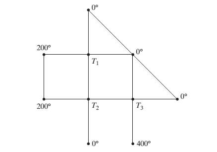
In a grid of wires, the temperature at exterior meshpoints is maintained at constant values (in °C), as shownin the accompanying figure. When the grid is in thermalequilibrium, the temperature T at each interior meshpoint is the average of the temperatures at the fouradjacent points. For example, T 2 = T 3 + T 1 + 200 + 0 4 . Find the temperatures T 1 , T 2 , and T 3 when the grid isin thermal equilibrium.
In a grid of wires, the temperature at exterior meshpoints is maintained at constant values (in °C), as shownin the accompanying figure. When the grid is in thermalequilibrium, the temperature T at each interior meshpoint is the average of the temperatures at the fouradjacent points. For example, T 2 = T 3 + T 1 + 200 + 0 4 . Find the temperatures T 1 , T 2 , and T 3 when the grid isin thermal equilibrium.
In a grid of wires, the temperature at exterior meshpoints is maintained at constant values (in °C), as shownin the accompanying figure. When the grid is in thermalequilibrium, the temperature T at each interior meshpoint is the average of the temperatures at the fouradjacent points. For example,
T
2
=
T
3
+
T
1
+
200
+
0
4
. Find the temperatures
T
1
,
T
2
,
and
T
3
when the grid isin thermal equilibrium.
A cup of water at an initial temperature of 81°C is placed in a room at a constant temperature of 24°C. The temperature of the water is measured every 5 minutes during a half-hour period. The results are recorded as ordered pairs of the form (t, T), where t is the time (in minutes) and T is the temperature (in degrees Celsius).
(0, 81.0°), (5, 69.0°), (10, 60.5°), (15, 54.2°), (20, 49.3°), (25, 45.4°), (30, 42.6°)
(a) Subtract the room temperature from each of the temperatures in the ordered pairs. Use a graphing utility to plot the data points (t, T) and (t, T − 24).
(b) An exponential model for the data (t, T − 24) is T − 24 = 54.4(0.964)t. Solve for T and graph the model. Compare the result with the plot of the original data.
(c) Use a graphing utility to plot the points (t, ln(T − 24)) and observe that the points appear to be linear.
Use the regression feature of the graphing utility to fit a line to these data. This resulting line has the form ln(T − 24) = at + b, which is…
In your Capstone software create a table with the following variables:
Position x, m: 1, 2, 3, 4
Coefficient of friction μ: 0.36
Velocity v, m/s: v=V 2. u.9.8.x
(b) Using clearly written arrows, indicate on each figure which grid curves correspond to u
being held constant, and which grid curves correspond to v being held constant. Write "u
constant" and "v constant".
10
05
200
-as
-1.0
FIGURE 1.
FIGURE 2.
0.5
-1.0
FIGURE 3.
FIGURE 4.
Need a deep-dive on the concept behind this application? Look no further. Learn more about this topic, algebra and related others by exploring similar questions and additional content below.


 Algebra: Structure And Method, Book 1AlgebraISBN:9780395977224Author:Richard G. Brown, Mary P. Dolciani, Robert H. Sorgenfrey, William L. ColePublisher:McDougal Littell
 Algebra & Trigonometry with Analytic GeometryAlgebraISBN:9781133382119Author:SwokowskiPublisher:Cengage